I finally had a chance to dig into the chipwhisperer. It’s a learning tool to teach about hardware security vulnerabilities like Side-channel attacks.

Years ago, my awesome wife saw my interest in a random Kickstarter, and supported it for my birthday. Turns out it was one of the better ones and it came through. Unfortunately, I was busy with work at the time, and didn’t have a chance to dig into it until now.

The tools and documentation are actually pretty good. However, at least for me, I got a little lost in the process. This is exacerbated by the fact that they recently (amazingly for a Kickstarter, they’re still doing active development years later) revamped the interface to the device. Most of the tutorials on their site are out of date, which makes things a bit confusing.

While the basic idea and first few tutorials are explained pretty well, things started becoming less clear around the 3rd tutorial. I ended up needing to get a copy of a textbook on the subject to understand some of the terms and unexplained details.

Overview

I’ll be talking about my experience setting up and using the chipwhisperer-lite, but it seems like they keep things consistent between hardware revisions for the most part.

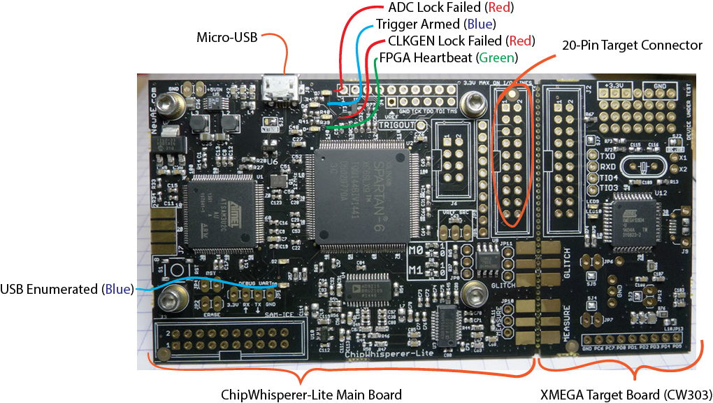
At a high level the board has two parts:

• An analyzer that uses an analog to digital converter (ADC) to measure power fluctuations
• A target board that acts like the victim to be “attacked”

For my board, the analyzer is a combination of a SAM3U USB interface chip and a Xilinx Spartan FPGA. The SAM3U acts as the interface to the computer. It implements a USB-3 interface to rapidly dump the captured data to the PC you’re running the analysis with. It has upgradable firmware, but there isn’t an obvious way to check it with the new interface tools. The FPGA is what actually interfaces with the ADC and does the low latency capture. It is programmed for each use, so it’s version is handled automatically as part of the rest of the tool chain.

The target board is an Atmel XMEGA microcontroller.

The goal of using the board is to configure the target board with some secret information (encryption keys), then use the analyzer to recover them.

Once you finish the learning process, you can actually break off the target board, and use the chip whisperer to analyze real hardware.

Getting set up

Depending on your system, there are many potential ways to get started. I went with their recommended easiest route using a VM.

Hardware

From my usage, there was zero hardware setup required. Just plugged it into my computer’s USB-3 port and didn’t need to do anything else.

Software

Following links from https://wiki.newae.com/V5:Getting_Started I eventually found https://chipwhisperer.readthedocs.io/en/latest/installing.html#install . At first it was a little confusing to understand what their toolchain actually was. Here’s my understanding:

Originally they had a dedicated GUI and API to interface with the hardware, and run analysis. In v5 they moved to using a Python API and supporting Jupyter notebooks https://jupyter.org/ as the recommended way to have a GUI.

So the software you need to set up is:

• Python environment with Jupyter Notebook
• API to communicate with analysis tools
• Compilers for target hardware
• Drivers for connecting to hardware

They provide instructions for setting this up on all major OS’s, but also provide a VM image with everything already set up.

This is pretty great, and I wish it was a more common way to distribute complex software tools.

I just needed to install the latest version of VirtualBox along with the extension pack (I created an issue for a little inconsistency in the documentation I ran into https://github.com/newaetech/chipwhisperer/issues/253 ). Then download and run the virtual machine image from the current gitub release https://github.com/newaetech/chipwhisperer/releases . https://chipwhisperer.readthedocs.io/en/latest/installing.html#install-virtual-machine gives instructions on logging in and setting a new password for the Jupyter Notebook. It took me a second to realize that I couldn’t tab complete reboot and needed to run sudo reboot.

Using the tools

With everything set up the VM runs Jupyter in the VM and makes the web server available on port 8888. I simply went to http://localhost:8888 in my browser and logged in. This let’s you get started with the actual tutorial by opening http://localhost:8888/notebooks/jupyter/!!Introduction_to_Jupyter!!.ipynb. Later I also accessed the Notebook from other computers by replacing localhost with my laptops LAN IP address.

This is then followed by http://localhost:8888/notebooks/jupyter/!!Suggested_Completion_Order!!.ipynb which gives you the list of “labs” to complete.

Labs

The labs are interactive Jupyter notebooks that you walk through. For the most part you just need to run each cell without modification, but occasionally you’ll need to modify some code. Most of the changes that I needed to make were to tune the parameters for my specific board.

You can see the notebooks along with there results at https://chipwhisperer.readthedocs.io/en/latest/tutorials.html

Lab 1 - Firmware Build Setup

http://localhost:8888/notebooks/jupyter/PA_Intro_1-Firmware_Build_Setup.ipynb https://chipwhisperer.readthedocs.io/en/latest/tutorials/pa_intro_1-openadc-cwlitexmega.html#tutorial-pa-intro-1-openadc-cwlitexmega

This lab lets you test your setup and get used to the tool chain basics. The only thing that wasn’t super clear for me, was that when they ask you to modify the firmware code, you can use your browser to go to: http://localhost:8888/tree/hardware/victims/firmware/simpleserial-base-lab1. To edit the firmware files you copied in a previous step.

Lab 2 - Capturing Data

http://localhost:8888/notebooks/jupyter/PA_Intro_2-Instruction_Differences.ipynb https://chipwhisperer.readthedocs.io/en/latest/tutorials/pa_intro_2-openadc-cwlitexmega.html#tutorial-pa-intro-2-openadc-cwlitexmega

This lab has you actually test a data capture.

It kind of violates the spirit of a notebook since you can’t just rerun the notebook when you’re done since you need to change the firmware code between steps.

I swapped the following code

1
for(volatile int i = 0; i  < 8 ; i++);

1
for(volatile int i = 1; i < 6561; i*=3);

I renamed the data collections and plotted them together with:

1
2
3
4
5
test1 = hv.Curve(trace_add.wave).opts(width=600, height=600, )
test2 = hv.Curve(trace_mult.wave).opts(width=600, height=600)
composition = test2 * test1
composition

Where orange is the addition and blue is the multiplication

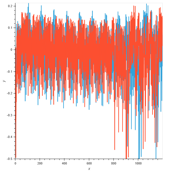
One thing that these labs don’t really cover, is how the multiple traces are being synced up so that they all line up in time for the programs execution. My understanding is that the target is outputting a sync signal to simplify this.

Lab 3 - Measuring SNR of the Target

http://localhost:8888/notebooks/jupyter/PA_Intro_3-Measuring_SNR_of_Target.ipynb https://chipwhisperer.readthedocs.io/en/latest/tutorials/pa_intro_3-openadc-cwlitexmega.html#tutorial-pa-intro-3-openadc-cwlitexmega

On a first run through, I couldn’t follow the explanation for this section. I googled around and started reading: https://www.iacr.org/archive/ches2004/31560016/31560016.pdf which sort of explained what’s going on, but I ended up needing to read the first four chapters of Power Analysis Attacks: Revealing the Secrets of Smart Cards to really understand what was happening.

I at least understood that DPA was for digital power analysis and HW was hamming weight. Part of the problem is that some of these concepts are explained more in other labs, but there’s a lot of interdependence. See my section on Power Analysis Attacks Textbook Notes for some of the terminology and assumptions I only understood after reading the textbook.

Even understanding the definition of SNR, the exact meaning is dependant on the specific attack being performed. Here’s how the SNR is calculated for this lab.

1. Generate 1000 text sequences and 1 encryption key.
2. Capture a trace of the target encrypting each text sequence.
3. Create a function to calculate the Hamming Weight of an intermediate value in AES algorithm (the sbox output)
4. Group the traces by the Hamming Weight of the intermediate value of the first byte being encrypted.
5. For each time point in the traces find the mean over all the traces with the same Hamming Weight.
6. Calculate the variance between these means (the variance across the different Hamming Weights is the signal).
7. Calculate the variance of each point in the trace for a single Hamming Weight (the noise)
8. Plot the signal/noise for the SNR

Lab 4 - Timing Analysis with Power for Password Bypass

http://localhost:8888/notebooks/jupyter/PA_SPA_1-Timing_Analysis_with_Power_for_Password_Bypass.ipynb https://chipwhisperer.readthedocs.io/en/latest/tutorials/pa_spa_1-openadc-cwlitexmega.html#tutorial-pa-spa-1-openadc-cwlitexmega

This one was a bit easier to understand. Basically, just monitoring the execution of code validating a password to find out how many instructions it takes to detect an incorrect byte for the password.

You guess all the possible bytes and look for which one causes a change in the power usage.

The initial values given didn’t work for me, so I had to spend a little time tweaking the analysis to get the right values for the checkpass function. Basically just looked at the timing results for the first two characters to get the offset and the spacing. Initially, I didn’t realize that I hadn’t chosen the very first divergence in the execution. This worked for all by the last character since getting the password correct caused a different execution path.

For my XMEGA I ended up with

return trace[69 + 36 * i] > -0.1 which I guess wasn’t too far off from the original return trace[73 + 40 * i] > -0.3

Lab 5 - Hamming Weight Measurement

http://localhost:8888/notebooks/jupyter/PA_DPA_1-Hamming_Weight_Measurement.ipynb https://chipwhisperer.readthedocs.io/en/latest/tutorials/pa_dpa_1-openadc-cwlitexmega.html#tutorial-pa-dpa-1-openadc-cwlitexmega

This is where I initially gave up and needed to create Power Analysis Attacks Textbook Notes before continuing.

In order to attack the AES algorithm we’re going to try to target a intermediate state that results when a byte of plaintext is X-ORed with the key and then sent through a lookup table called the S-BOX. The idea that since this point is a function of both the input and the key it can be used to deduce the key. I’m not clear on why this point is used instead of the output of the X-OR, but it might have to do with which states are being output onto the data bus. We then build a function to map the data and key to the S-BOX output, and for looking up the Hamming Weight (HW) of a byte. The last step in this section is to look at a plot of the trace for a region where it should be doing the AES calculation. The traces are then color coded by the HW of the first byte. I’m not really sure why this plot is chosen, since you don’t know which point corresponds to the byte 0 you calculate the HW for.

We average across the traces that share a HW for each time point. We sort each trace by the HW of the first byte of the S-BOX output and average the traces with this HW. Then we find the correlation of each point with the means from each HW. Basically is the HW from 0-9 linearly correlate to the mean power for a point. When I ran this I had a high correlation with a point way outside the range given for my hardware target. Looking at the plot of the point also didn’t show nearly as clear a gradient as the example.

Regardless the point is relatively linear and shows the general approach we’re taking works.

Lab 6 - Large HW Swings

http://localhost:8888/notebooks/jupyter/PA_DPA_2-Large_HW_Swings.ipynb https://chipwhisperer.readthedocs.io/en/latest/tutorials/pa_dpa_2-openadc-cwlitexmega.html#tutorial-pa-dpa-2-openadc-cwlitexmega

This conceptually is a somewhat simpler version of the last lab. Instead of dealing with S-BOX output of random keys and data, it instead limits the first byte of data to either be randomly 0 or 0xFF.

This means that a simple diff between the mean of traces with 0, and the mean of traces with 0xFF shows an obvious spike when the value is being processed. It’s interesting these peaks don’t match with the high correlation points from the previous lab, since they should both be showing correlations with the first data byte.

Lab 7 - AES DPA Attack

http://localhost:8888/notebooks/jupyter/PA_DPA_3-AES_DPA_Attack.ipynb https://chipwhisperer.readthedocs.io/en/latest/tutorials/pa_dpa_3-openadc-cwlitexmega.html#tutorial-pa-dpa-3-openadc-cwlitexmega

Big warning at the top of the lab that this attack is less reliable on my target platform.

Pretty similar to previous couple labs, except using the principles to actually deduce the key. I’m a little confused since each trace is still using a random key. On closer examination it turns out fixedKey is true by default, so the known_keys for each trace should be the same.

After the long processing period the algorithm got 8/16 bytes of the key correct.

Let’s see if I can understand the analysis.

1. The attacks on each subkey byte are independent from each other and performed one after the other.
2. The analysis goes through all 256 possible values for the subkey byte
3. Each trace is classified into a list based on whether the SBOX output dependent on the subkey byte will produce a result with 1 as the least significant bit (one_list) or 0 (zero_list).
4. The mean of the traces for each time point is taken and the difference for each time point between the one_list and zero_list is taken.
5. The time point with the largest absolute difference is found, and this difference value is recorded for the subkey guess.
6. Once all the subkeys have been checked the keyGuess with the largest power difference between the one_list and zero_list is recorded as the best.

Once I understood this I found it strange that they were just looking at a single byte of the SBOX output. I wondered if I’d get better results with a different comparison. I understood they used a single bit so they could separate the traces into two buckets, but it seems like there are more effective comparisons. First I tried only considering traces where the SBOX was either 0 of 0xFF, but this wasn’t finding any keys. This was probably since it was limited to 1/128 the number of data points. Next I classified the traces as having the SBOX output having a HW of either <4 or >4. This left out the traces where 4 was the hamming weight, but still seemed to be a big improvement. With this change the algorithm was able to find the entire 16 byte key.

1
2
3
4
5
6
7
8
9
10
11
12
13
14
15
16
17
18
19
20
21
22
23
24
25
26
27
28
29
30
31
32
33
34
35
from tqdm import tnrange
import numpy as np
mean_diffs = np.zeros(255)
key_guess = []
# key used for all traces
known_key = known_keys[0]
plots = []
HW = [bin(n).count("1") for n in range(0, 256)]
# index 0-15 of the byte of the key we're attacking
for subkey in tnrange(0, 16, desc="Attacking Subkey"):
    # for each subkey try every possible byte value
    for kguess in tnrange(255, desc="Keyguess", leave=False):
        one_list = []
        zero_list = []
        # based on the byte corresponding with the subkey
        # clasify the S-Box output as having a HW > or < 4
        for tnum in range(numtraces):
            if (HW[intermediate(textin_array[tnum][subkey], kguess)] > 4 ):
                one_list.append(trace_array[tnum])
            elif (HW[intermediate(textin_array[tnum][subkey], kguess)] < 4):
                zero_list.append(trace_array[tnum])
        # Average the traces based on the HW of the SBOX output
        one_avg = np.asarray(one_list).mean(axis=0)
        zero_avg = np.asarray(zero_list).mean(axis=0)
        # Find the point with the largest difference between the traces in the two HW buckets
        mean_diffs[kguess] = np.max(abs(one_avg - zero_avg))
        if kguess == known_key[subkey]:
            plots.append(abs(one_avg - zero_avg))
    # Get the guess that had the largest diff
    guess = np.argsort(mean_diffs)[-1]
    key_guess.append(guess)
    print(hex(guess) + "(real = 0x{:02X})".format(known_key[subkey]))
    #mean_diffs.sort()
    print(mean_diffs[guess])
    print(mean_diffs[known_key[subkey]])

Conclusion

There’s more labs to go, but I decided to stop here for now. It was a lot of fun to get back into something resembling a college lab course complete with required reading.

The software and hardware for the ChipWhisperer did a great job of making the process simple and convenient.

The main challenge was the documentation. The recent refactor made finding the relevant information much harder. Also, there was some pretty huge jumps in assumed background knowledge between the labs. Having clearer links to further reading, or at least defining terms when they were first used would make following what’s going on a lot easier. This is coming from someone with a lot of existing background in these areas. It would probably be impenetrable to someone without some of this context.

While I don’t think I could go out and perform a DPA attack on some random processor I have lying around (the textbook explains a lot of the challenges that attacking an unknown hardware poses) I at least feel like I have a pretty firm grasp on the basic principles.

Power Analysis Attacks Textbook Notes

Chapter 1 Intro

high level overview of what we’re trying to do. How the internal state of an encryption algorithm produces intermediate values that reflect the values of encryption keys, and how we can potentially correlate power measurements to learn what the processor is doing.

Chapter 2 Crypto devices

Overview of the hardware that can make up a crypto device. Goes into some detail on how a chip made with CMOS technology works on the transistor level.

Chapter 3 Power Consumption

• Focusing on CMOS devices, talks about how the power usage is the static plus the dynamic effects of a complementary gate switching from 1->0 or 0->1.
• The factors of the dynamic power are the charging current (current to charge the capacitance inherent in the transistors and the attached wiring). This power use only happens from 0->1 transitions and us a function of the voltage, frequency, and capacitance of the circuit.
• Another power use is the short circuit current for the brief period a short circuit is created when the gates flip. This occurs in both transitions.
• Another use is glitches. These are the intermediate states caused by signals not traveling through combinational logic all at the same rate. This can cause gates to flip back and forth in between clock cycles.
• Hamming distance model - count the number of 0->1 and 1->0 transitions during a time interval. This is then used to describe the power usage. It assumes that all the transitions and cells cause equal power draw along with other simplifications. Hamming distance is the XOR of the Hamming weight (the number of bits set to 1) between two states.

  The Hamming-distance model assumes that all cells contribute to the power consumption equally and that there is no difference between 0 -> 1 and 1 -> 0 transitions. The Hamming distance between two values Vo and VI can be calculated as follows: HD( Vo, VI) = HW( Vo XOR VI)

• As an attacker knowledge of the device under attack is limited, and assumptions need to be made. For a microcontroller a common assumption is that a databus is part of it’s design. This bus is well modelled by the Hamming Distance.
• This is especially true since an attacker often knows consecutive values. This means registers are also a good target.
• Hamming-Weight model, a simplification of the HD model where the attacker only knows a single value, not consecutive. It assumes the power use is proportional to the number of set bits. Ideally the value before the observed state is 0, or at least a constant value for each test.
• The rest of the chapter goes on to describe the real world challenges for capturing the power used by ASIC and CPU base encryption. Most importantly it describes the basic set up of attaching a clock and power to a device under attack and using an oscilloscope to measure the power drop over a 1olm resistor. The paper talks about using a sync signal to line up the repeated sampling of the computation.

  Chapter 4 statistical characteristics of a trace

• Here a trace is a time series of captured voltages.
• Each point of a power trace can be modeled as the sum of an operation dependent component Pop, a data-dependent component Pdata, electronic noise Pel. noise, and a constant component P const.
• We can use these components to analyse a single point in time across traces. Here we care about Pop, Pdata, and Pnoise. We can estimate the noise by looking at a point with the same operation and data. The noise is Gausian and we can calculate the mean and StdDev.
• You can also look at a single point as it processes different data values and look at the histogram of power usage. If you go through all 256 data values you get a histogram that is the sum of 9 different normal functions (corresponding to the 9 hamming weights (0-8)).
• The hamming weight of uniformly random 8 bit value is a binomial distribution (set bits in 0,1,2,etc.)
• The operation being performed also affects power. This may or may not be independent of the Pdata.
• The measurement of information leakage is the SNR. This is specific to an attack scenario. The signal is notated as the Pexp or the exploitable power usage.
• Since there can be noise component due to switching of bits that aren’t the focus of an attack is Pop + Pdata = Pexp + Psw.noise or Ptotal = Pexp + Psw.noise + Pel.noise + Pconst
• Psw.noise can be estimated by keeping the bits of interest constant and uniformly varying the other bits. This distribution can then be aproximated as Gaussian
• SNR = Var(signal) / Var (noise) for a becomes Var(Pexp) / (Var(Psw.noise + Pel.noise))
• In addition to looking at single points in the power trace, correlation between points is another way to look at data.
• The correlation coefficient measures the linear relationship between two variables. It is always between -1 and 1.
• This can be expanded to view the trace as a multivariate gaussian to look for the correlation matrix between the points on the trace.